on
Post Election Reflection Model
Welcome to my 2022 Midterm blog series. I’m Kaela Ellis, a junior at Harvard College studying Government. This semester I am taking Gov 1347: Election Analytics taught by Professor Ryan Enos, which has led to the creation of this blog. The goal of this blog series is to predict the 2022 Midterm election. With this blog series I predicted that Democrats would win 45.58466% of the vote share. While some of the election results are still contested, as of 11/21/2022, the Democrats won 48.32% of the popular vote.
## [1] 45.58466## Model Fit lwr upr
## 1 Dem Prediction 45.67219 42.77461 48.56978
## 2 Rep Prediction 54.32781 51.43022 57.22539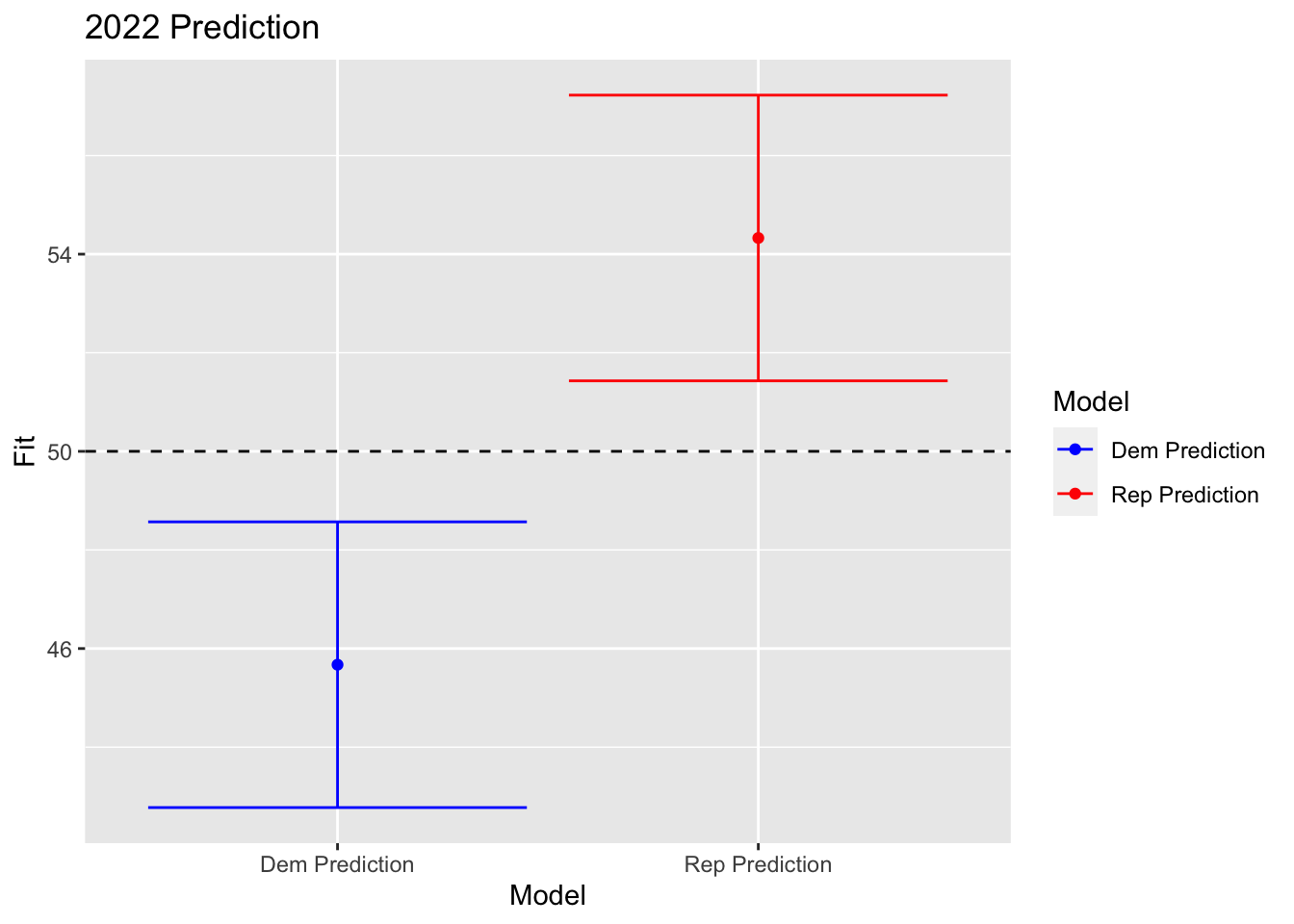 In my forecast model, I used four variables from only midterm years dating back to 1954: approval rating, consumer sentiment, generic ballot, and incumbency. My model was formatted around predicting the incumbent party’s vote share largely because of retrospective voting theory. Under this theory, voters use elections to hold incumbents accountable; so, if their welfare has decreased, they won’t reelect the incumbent. Therefore, I compared the consumer sentiment and presidential approval rating to the incumbent president’s vote share. Using my four indicators, I obtained an R2 of 0.714, and a Democratic party loss of 45.58466% of the vote share. This prediction was 2.74% points lower than the actual Democratic two-party vote share of 48.32%. The prediction does fall in my predicted range, as my upper bound is 48.57%. However, my prediction was still significantly off, and in the remainder of this post I will examine different reasons for this result.
## Warning in mean.default(President): argument is not numeric or logical:
## returning NA

## Warning in mean.default(President): argument is not numeric or logical:
## returning NA

## Warning in mean.default(President): argument is not numeric or logical:
## returning NA

## Warning in mean.default(President): argument is not numeric or logical:
## returning NA

## Warning in mean.default(President): argument is not numeric or logical:
## returning NA

## Warning in mean.default(President): argument is not numeric or logical:
## returning NA

## Warning in mean.default(President): argument is not numeric or logical:
## returning NA

## Warning in mean.default(President): argument is not numeric or logical:
## returning NA

## Warning in mean.default(President): argument is not numeric or logical:
## returning NA

## Warning in mean.default(President): argument is not numeric or logical:
## returning NA

## Warning in mean.default(President): argument is not numeric or logical:
## returning NA

## Warning in mean.default(President): argument is not numeric or logical:
## returning NA

## Warning in mean.default(President): argument is not numeric or logical:
## returning NA

## Warning in mean.default(President): argument is not numeric or logical:
## returning NA

## Warning in mean.default(President): argument is not numeric or logical:
## returning NA

## Warning in mean.default(President): argument is not numeric or logical:
## returning NA

## Warning in mean.default(President): argument is not numeric or logical:
## returning NA

## Warning in mean.default(President): argument is not numeric or logical:
## returning NA
## Warning in mean.default(Party): argument is not numeric or logical: returning NA
## Warning in mean.default(Party): argument is not numeric or logical: returning NA
## Warning in mean.default(Party): argument is not numeric or logical: returning NA
## Warning in mean.default(Party): argument is not numeric or logical: returning NA
## Warning in mean.default(Party): argument is not numeric or logical: returning NA
## Warning in mean.default(Party): argument is not numeric or logical: returning NA
## Warning in mean.default(Party): argument is not numeric or logical: returning NA
## Warning in mean.default(Party): argument is not numeric or logical: returning NA
## Warning in mean.default(Party): argument is not numeric or logical: returning NA
## Warning in mean.default(Party): argument is not numeric or logical: returning NA
## Warning in mean.default(Party): argument is not numeric or logical: returning NA
## Warning in mean.default(Party): argument is not numeric or logical: returning NA
## Warning in mean.default(Party): argument is not numeric or logical: returning NA
## Warning in mean.default(Party): argument is not numeric or logical: returning NA
## Warning in mean.default(Party): argument is not numeric or logical: returning NA
## Warning in mean.default(Party): argument is not numeric or logical: returning NA
## Warning in mean.default(Party): argument is not numeric or logical: returning NA
## Warning in mean.default(Party): argument is not numeric or logical: returning NA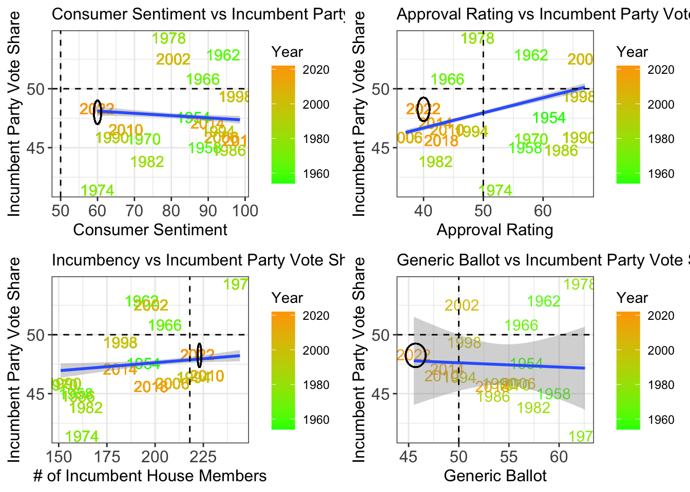 In the above models, I plotted the accuracy of each of my indicators. Looking at consumer sentiment, 2022 is not a novelty year. With a consumer sentiment of 59.9, its vote share falls directly on the trend line. Again, with approval rating, 2022 is relatively close to the line. With incumbency, which is a measure of the number of incumbent members running, 2022 again falls on the trend line. This same relationship is seen with the generic ballot. Based off of my four indicators 2022 does not seem to be a novelty year. However, when I examine these four graphs more closely, I notice a historical trend: the more recent the year, the closer it is to the trend line, and the less recent the year, the higher the likelihood of it being an outlier. Using a color scale, I visually represented this: the more recent the year, the more orange the year’s color is, and the less recent the year, the more green the year’s color is. The outliers tend to be green on all of these graphs. Therefore, I hypothesized that in my attempts to have more data points, I included old years that threw off the accuracy of my model.
## [1] 47.14827## model_recent Fit lwr upr
## 1 Dem Prediction 45.67219 42.77461 48.56978
## 2 Rep Prediction 54.32781 51.43022 57.22539So, I tested this hypothesis. I removed half of the year from my dataset – all of the years that were green, which was any year prior to 1986. I reran my prediction model, and my prediction changed to 47.14%. This is significantly closer to the election results. Adding this variable also bumped my R2 up from 0.714 to 0.752. If I were to predict the election again, I would not include the years 1954 through 1986. It seems that these older years skewed toward inaccuracies. Through this statistical finding, I can make the inference that the American political landscape has changed to the extent that the way voters are affected by fundamentals has changed.
I think another issue I had throughout this course was adjusting my predictions to match popular forecasters. I assumed that the forecasters, such as the Economist and Five-Thirty-Eight, were right and based the accuracy of my prediction off of their predictions. This created biases in my model. I cannot test the effect of this bias, but it is something to keep in mind.
Another potential flaw in my model was that I used incumbency as my model base, rather than party, meaning I measured how my variables interacted with the incumbent party vote share, rather than how they interacted with the Democratic or Republican party. My model assumed that the Democratic and Republican vote shares reacted the same to fundamentals. However, this is not true. For example, in my blog 3 post, I found a positive relationship between the consumer sentiment and Republican party vote share. However, when I performed the same test for the Democratic party, I found a negative relationship between consumer sentiment and the Democratic party vote share. This may indicate that voters attach certain fundamentals to certain parties. My statistical tests on consumer sentiment suggest that voters use economic fundamentals to evaluate the Republican party, but not the evaluate the Democratic party. Therefore, I hypothesize that I should have incorporated a party variable into my model.
## [1] 45.47081## model_party Fit lwr upr
## 1 Dem Prediction 45.67219 42.77461 48.56978
## 2 Rep Prediction 54.32781 51.43022 57.22539I tested my hypothesis by creating a party indicator. The coefficient of this variable when input into the overall prediction model was -0.419 – it was my only negative coefficient. This means that every time a Democrat is an incumbent, they lose an average of 0.419. I can find no obvious logical reason for this, and therefore question this variable. It slightly improved the R2 of the overall model from 0.714 to 0.721. However, this R2 increase is likely simply a proxy of adding an additional variable, which leads to overfitting. My prediction also became less accurate with a Democratic vote share of 45.47. Therefore, the interaction between my four variables and the party seems to have minimal effect, if any.
One change I would make to my prediction model would be incorporating a previous election vote share variable. This would serve as a stabilizer in my model. Being that the political climate usually does not drastically change every two years, and it is usually more of a gradual change, I thought that this would be an indicator. I added the variable of previous election vote share to my model. Since I took the vote share from presidential elections, this was the first variable that used data from presidential election years.
all.not.2022 <- subset(all.and.2022, Year < 2022)
lm_all_previous_VS <- lm(Vote_Share ~ Approval_Rating  + consumer.sentiment + incumb_poll + Incumbent + Previous_vote_share, data = all.not.2022)

data.20$Previous_vote_share <- 51.5

model_previous_VS <- predict(lm_all_previous_VS, data.20, interval="prediction")
mean(model_previous_VS)
## [1] 45.45344interval <- data.frame("model_previous_VS" = character(), # Create empty data frame
"Fit" = numeric(),
"lwr" = numeric(),
"upr" = numeric(),
stringsAsFactors = FALSE)
interval[1, ] <- list("Dem Prediction", model[1,1], model[1,2], model[1,3])
interval[2, ] <- list("Rep Prediction", model_Rep[1,1], model_Rep[1,2], model_Rep[1,3])
interval$lwr <- as.numeric(interval$lwr)
interval$Fit <- as.numeric(interval$Fit)
interval$upr <- as.numeric(interval$upr)
print(interval)## model_previous_VS Fit lwr upr
## 1 Dem Prediction 45.67219 42.77461 48.56978
## 2 Rep Prediction 54.32781 51.43022 57.22539The effect of including the previous vote share is minimal if any. The R2 of my model slightly increased from 0.714 to 0.717. The accuracy of my prediction decreased, as my forecast with this variable is Democrats securing 45.45% of the national vote share. Therefore, this hypothesis was wrong. If I were to predict the election again, I would still not include this variable.