on
Blog_Post_6
Welcome to my 2022 Midterm blog series. I’m Kaela Ellis, a junior at Harvard College studying Government. This semester I am taking Gov 1347: Election Analytics taught by Professor Ryan Enos, which has led to the creation of this blog. I will use this blog series to predict the 2022 Midterm election. The series will be updated weekly with new predictive measures and analyses of past elections.
This week I decided to incorporate turnout, incumbency, and expert predictions into my district-level two-party vote share prediction. As we saw from previous weeks campaigns do three things: persuade voters to support their candidate, turnout voters to support their vote, and convince voters to donate. Campaigns are not very effective in persuading voters to support their candidate. They have greater efficacy when trying to increase voter turnout. For example, as the Enos and Fowler reading found, the Obama campaign in 2012 increased voter turnout by approximately 8 percentage points, showing that campaigns have the potential to increase turnout by 8 points.
However, some of the readings from this week also explored the drawbacks of ground game efforts. For example Enos and Hersh point out that canvassers are more ideologically extreme and have different policy priorities than the median voter. They point out that canvassers are likely so ideologically extreme because citizens who have ideological extremes gain more utility in pushing their extreme positions. Additionally, partaking in political activism can make one more polarized. Enos and Hersh found that 73% of the mass public thought that the economy was the most important issue, while less than 40% of canvassers thought so. This demonstrates how canvassers have different policy priorities. This leads to a principal-agent problem, as candidates have limited control over volunteer canvassers. As a result of factors such as these, Enos and Hersh found that voters contacted by in-person Obama canvassers were less likely to support Obama, demonstrating a backfire effect.
This week I used voter turnout as a proxy for turnout. I worked on some of the code for this blog post with Lucy Ding and Jude Park. We created a district-by-district forecast, including the variables: average support, turnout, GDP, and incumbency. I used these variable in the model as follows:
I calculated district level turnout by adding the Republican vote share and adding it to the Democratic vote share, and then dividing it by the current voting age population (CVAP). While this is not necessarily the best way to predict turnout, we have the most readily available data on this. The main drawback to using this I found was that I could only find data on turnout tracking back to 2012. This is clearly very limited, as it only gives me 5 points of data to predict my forecast off of. With less points of data, the accuracy of my forecast is limited. Other methods for calculating turnout that would be more reflective of ground game efforts would be a measure of some of the factors that Gerber and Green discussed in their 2015 paper. They discussed how get out the vote efforts that emphasized one’s civic duty, polling place location, and reminder of an early pledge to vote are statistically proven to increase voter turnout. Meanwhile other GOTV efforts, such as leaflets, signage, direct mail reminders, and emails, have no apparent effect. A measure of the effective GOTV methods may inform how campaign efforts can effect election turnout more accurately. However, this data is not accessible, and therefore I defaulted to using the CVAP.
To calculate average support, I averaged the generic ballot for 52 days prior to the election. I have discussed this decision in earlier blog iterations in greater detail. I may pivot to using a different metric in my final calculation, but the general thought here was that generic ballots closer to the election are more accurate and, therefore, better predictors of the election results.
To calculate the economic factor, I used quarter 6 to 7 difference for GDP. Again, I have discussed different metrics for determining the economic effect. This is not the best economic factor, and I may pivot in my final calculation, but my thought here was that the change in GDP from Q6 to Q7 is the most recent, and, therefore, the most salient.
For incumbency, I calculated whether or not the Democratic party was the incumbent. I have discussed this decision in past blog iterations, but the general thought here was that there is an incumbency advantage, and to calculate its affect on the Democratic vote share I code for incumbency in a 0:1 form.
## Reading layer `districts114' from data source
##   `/private/var/folders/53/y4tjcyz17pq_kfwb17bygwvm0000gp/T/RtmpuapeHx/districtShapes/districts114.shp'
##   using driver `ESRI Shapefile'
## Simple feature collection with 436 features and 15 fields (with 1 geometry empty)
## Geometry type: MULTIPOLYGON
## Dimension:     XY
## Bounding box:  xmin: -179.1473 ymin: 18.91383 xmax: 179.7785 ymax: 71.35256
## Geodetic CRS:  NAD83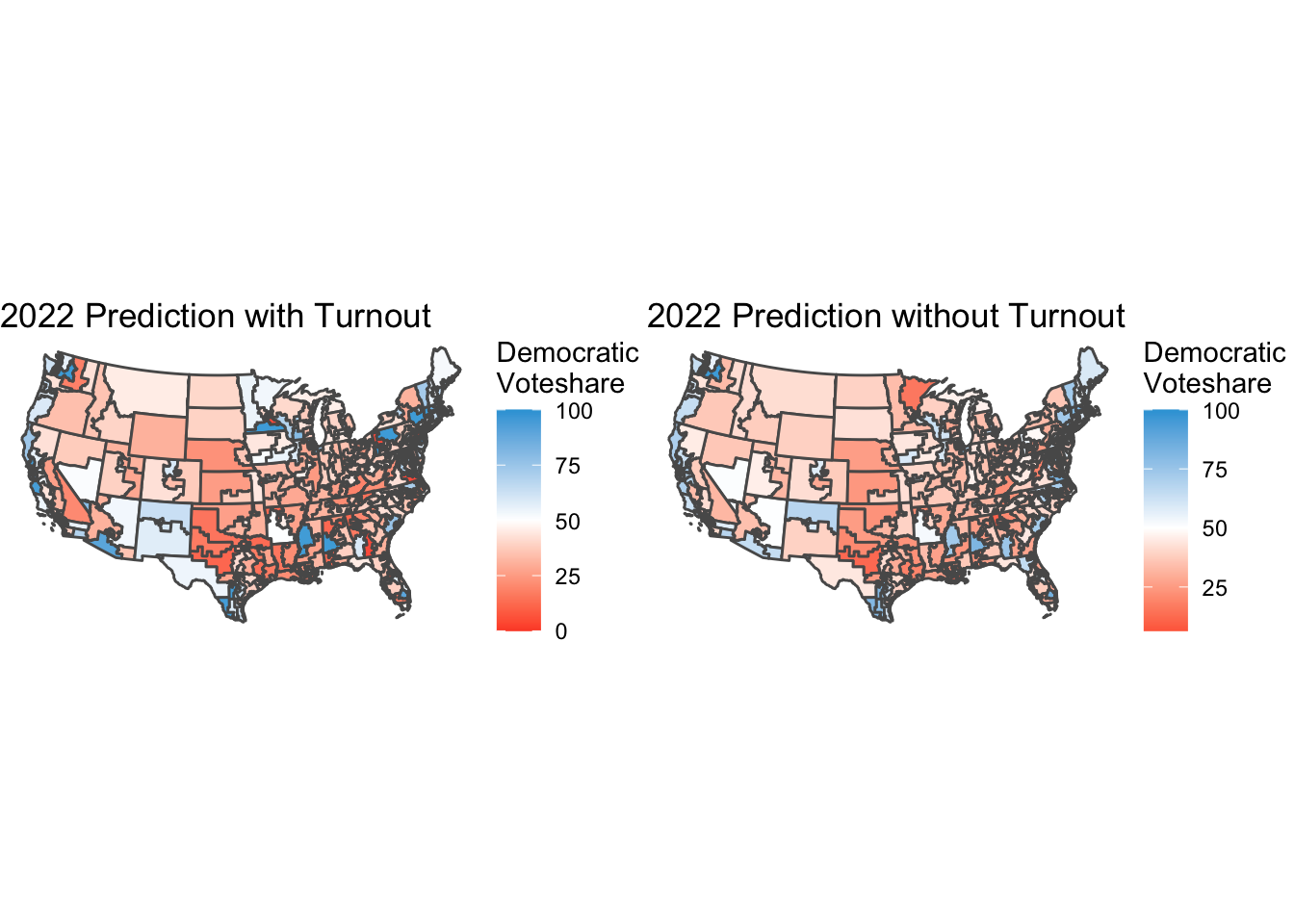
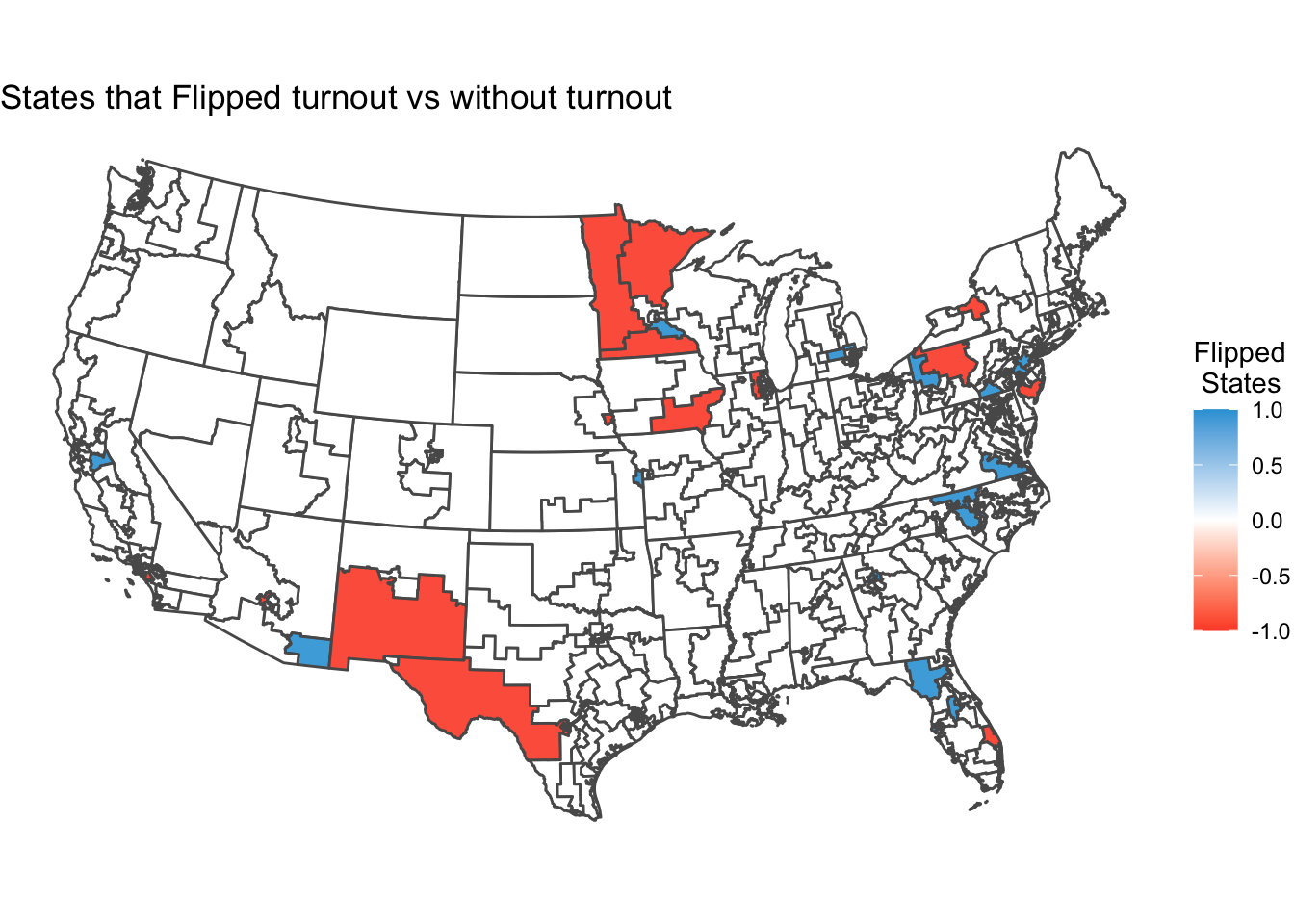 With the incorporation of incumbency into my model, I saw 36 states flip. So turnout had an affect on my predictions. With the turnout variable, I predict that Democrats will receive 220 seats.
Data
Model with Turnout
## [1] "5600"##
## ==================================================
## Dependent variable:
## ---------------------------
## DemVotesMajorPercent
## --------------------------------------------------
## average_support 1.347
## (1.397)
##
## turnout 0.089
## (0.313)
##
## gdp_percent_difference -0.379
## (0.323)
##
## incumb
##
##
## Constant -36.698
## (60.562)
##
## --------------------------------------------------
## Observations 5
## R2 0.614
## Adjusted R2 -0.544
## Residual Std. Error 4.485 (df = 1)
## F Statistic 0.530 (df = 3; 1)
## ==================================================
## Note: *p<0.1; **p<0.05; ***p<0.01## [1] 221## [1] 214## [1] 224## [1] 211## [1] 215## [1] 220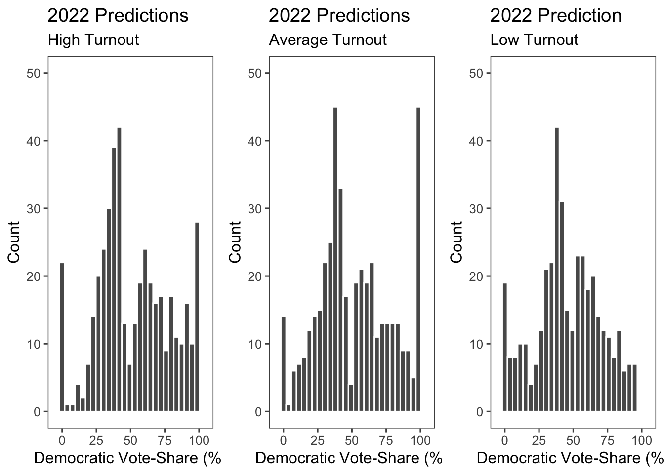 I then calculated how a change in the level of turnout would change the election results. I did the most extreme turnout change of 8%, since Enos and Fowler found that campaigns have the potential to effect turnout by 8 percentage points. I found that low turnout benefits Democrats, as they win the house majority with 220 seats. Then, with average turnout, Republicans take the house majority with 221 seats. Finally, with high turnout, Republicans have house majority with 224 seats.
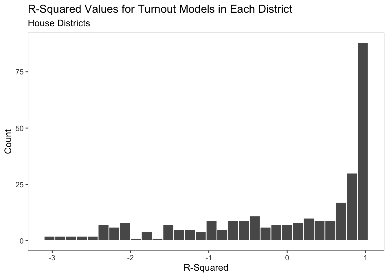 I then graphed the R2 values of the model for each state. Most of the values were close to 1, indicating that this is a decent model. This model shows the R2 for the forecast which includes all the variables. However, when I isolate R2 of turnout it is 0.089, which is not a statistically significant R2 value. Therefore, in later iterations of my model I likely will remove turnout from the model.