on
Blog Post 3
Welcome to my 2022 Midterm blog series. I’m Kaela Ellis, a junior at Harvard College studying Government. This semester I am taking Gov 1347: Election Analytics taught by Professor Ryan Enos, which has led to the creation of this blog. I will use this blog series to predict the 2022 Midterm election. The series will be updated weekly with new predictive measures and analyses of past elections.
This second third post examines the question of the effect of polls in predicting House elections. In particular, I look to see how the polls affect the predictivity of the popular vote, and how different methods of weighting and interpreting polls lead to different predictions. I will evaluate the Economist’s G.Elliot Morris’ and Nate Silver’s approach to forecasting models.
Morris and Silver take into account a lot of the same factors in making their forecasts. They both take into account the incumbent advantage, past voting records in Congress, presidential, candidate funding, polls timing, and a plethora of other factors.
One of Elliot Morris’ strong suits in poll forecasts- an area that Nate Silver seems to neglect- is accounting for how district-level votes usually do not follow a bell curve model; a forecast does not usually have an equal tendency to lean left or right. Therefore, Morris uses a skew-T to account for distributions with long tails. Another factor specific to Morris is his consideration of the midterm penalty- parties tend to lose votes in the election after they win the White House. Morris’ model factors in uncontested races, and it is unclear if Silver’s model does the same.
Silver emphases partisanship more. He explains how the more partisan the state is the more predictive it is, removing emphasis on candidate qualities. He also emphasizes district specific funding, being that he weighs funds raised in the candidate’s state as 5 times as valuable as funds raised outside of the state. Specific to the Silver model the CANTOR, a program that fills in states with missing information by using polling data from other states with similar demographic, geographic, and political factors. Silver doesn’t have ad-hoc adjustments to his forecasts, but he does have ad-hoc adjustments to his error models. For example, he factored in covid in the error of his forecast.
I think that Morris has the superior model. One of the major things that Morris considers where Silver lags is Morris’ specification on particular biases, while Silver tends to generalize. Morris looks at polls on the individual level. For example, if a poll consistently leaned left to a certain percent, Morris takes that into account. Whereas Silver tends to generalize by creating a house effect which adjusts the bias for partisan polls by 4 percentage points. According to Galton, if the polls are equally diverse on both ends- for example, there are an equal number of democrat polls and republican polls, then they should equal out to the correct average. However, Silver seems to be inserting that arbitrary generalized number of 4 percentage points for all partisan polls, failing to take into account how all polls have a specific level of bias specific to that poll. Thus, I think Morris’ approach is better in this way.
##Economic Factors
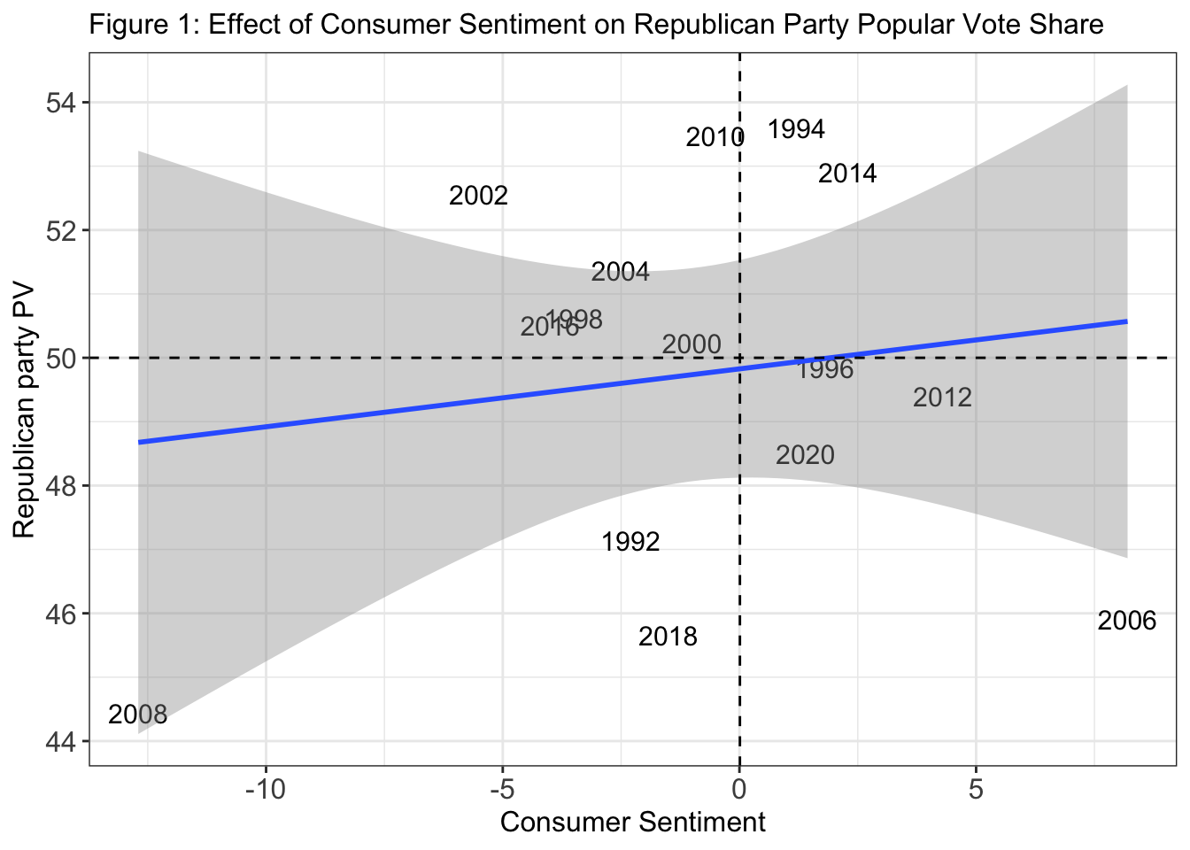 Before factoring in polls to my forecast, I returned to my economic indicators to improve my low R2 value. In the model above, I used consumer sentiment to inform my forecast. In John Tesler and Lynn Vavreck’s “The Electoral Landscape of 2016”, they explain that consumer sentiment is the best measure of Americans’ views of the economy. I therefore decided to use consumer sentiment as my economic indicator. I only looked at dates post 1992 because that is the last year before the Democrats lost control of the house, after holding it for many cycles. I also took the change in consumer sentiment from the month of September to October because the months closest to the election are the most salient. Additionally, instead of measuring how the incumbent party is rewarded or punished for economic indicators, I measured how the republican party is affected, as informed by discussions in class. I found a direct correlation between the consumer sentiment and the republican party’s vote share, however my R2 value continued to indicate statistical insignificance with an R2 of 0.022. In later weeks, I will again return to the economic indicator and continue to alter it to maintain a statistically significant value.
##polls
Before factoring in polls to my forecast, I returned to my economic indicators to improve my low R2 value. In the model above, I used consumer sentiment to inform my forecast. In John Tesler and Lynn Vavreck’s “The Electoral Landscape of 2016”, they explain that consumer sentiment is the best measure of Americans’ views of the economy. I therefore decided to use consumer sentiment as my economic indicator. I only looked at dates post 1992 because that is the last year before the Democrats lost control of the house, after holding it for many cycles. I also took the change in consumer sentiment from the month of September to October because the months closest to the election are the most salient. Additionally, instead of measuring how the incumbent party is rewarded or punished for economic indicators, I measured how the republican party is affected, as informed by discussions in class. I found a direct correlation between the consumer sentiment and the republican party’s vote share, however my R2 value continued to indicate statistical insignificance with an R2 of 0.022. In later weeks, I will again return to the economic indicator and continue to alter it to maintain a statistically significant value.
##polls
## [1] 51.38605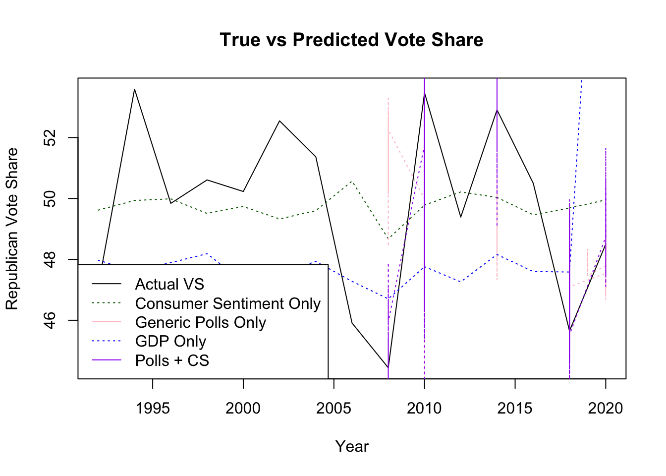
##
## Results
## =========================================================================================================================
##                                                                     Dependent variable:
##                                    --------------------------------------------------------------------------------------
##                                                                       R_majorvote_pct
##                                            CS                 Gpolls                 GDP               Gpolls + CS
##                                           (1)                   (2)                  (3)                   (4)
## -------------------------------------------------------------------------------------------------------------------------
## Consumer Sentiment                       0.091                                                           0.825***
##                                         (0.167)                                                          (0.028)
##
## Generic Polls                                                0.329***                                    0.616***
##                                                               (0.034)                                    (0.025)
##
## GDP                                                                                 0.827
##                                                                                    (0.642)
##
## Generic Polls + Consumer Sentiment     49.826***             32.860***            47.150***             20.072***
##                                         (0.788)               (1.633)              (0.701)               (1.173)
##
## -------------------------------------------------------------------------------------------------------------------------
## Observations                               15                   670                   35                   670
## R2                                       0.022                 0.124                0.048                 0.613
## Adjusted R2                              -0.053                0.123                0.019                 0.611
## Residual Std. Error                 2.990 (df = 13)      3.419 (df = 668)      3.093 (df = 33)       2.276 (df = 667)
## F Statistic                        0.293 (df = 1; 13) 94.976*** (df = 1; 668) 1.658 (df = 1; 33) 527.214*** (df = 2; 667)
## =========================================================================================================================
## Note:                                                                                         *p<0.1; **p<0.05; ***p<0.01
I then looked at Generic polls post 1992 during Congressional election years only. I used their tendency for error to indicate the error in the 2022 election, so that I can adjust them to predict the 2022 midterm. As Silver and Morris have shown there are many different ways to weigh polls. I took a more basic approach and examined polls on a national, rather than a state or district level. I will approve this in later weeks, focusing more on state or district level data. Using the generic polls alone, the predictivity of my model had a low R2 of 0.124, indicating that it is not a highly statistically significant model. However, when I combined the generic polls with the consumer sentiment data, my models became statistically significant with an R2 of 0.613. Using the polls and consumer sentiment together has shown to produce a more statistically significant prediction. Again, I aim to improve this statistical significance in later iterations of the blog, as I begin to further specify my data and add more indicators. My forecast using these two indicators is that the Republicans will receive 51.39% of the vote share.